15 min read
The NK model, step by step, with nkscape
- NK model
- Agent-based modeling
- Python
- Open source

Last week I published nkscape, a Python library for Kauffman NK fitness landscapes and NK-based agent-based models of organizations. It is open source under the MIT licence and on PyPI:
pip install nkscape
The library is the short part of this post. The long part is what an NK model is, the way I learned it before writing a line of code: with a firm that has three decisions, tables you can check by hand and one cube.
nkscape in short
A model consists of a landscape, agents and population rules. The landscape holds N binary decisions, an interaction matrix that says which decisions affect which payoffs, and random payoff tables. An agent is the search rule of one organization; you subclass it and write one method. A population rule, such as selection or a central choice, is applied to the whole population once per period. nk.run runs the periods and records every configuration, its fitness and who was alive.
There is no global random state: every function takes a seed, and an agent walks the same way alone as in a crowd. For N up to 24 the library holds the fitness of all 2^N configurations at once, so peaks and the global maximum are exact. It is tested, typed and documented, and a notebook reproduces Figures 1 to 9 of Levinthal (1997).
import nkscape as nk

landscape = nk.Landscape.next_k(10, 3, rng=42)  # N = 10 decisions, K = 3
print(landscape.count_peaks())  # 14

agents = [nk.agents.HillClimber("first") for _ in range(100)]
result = nk.run(landscape, agents, periods=20, rng=1)
print(result.fitness[:, -1].mean() / landscape.global_max())  # 0.944
A firm with three decisions
Picture a small firm facing three decisions, each answered with 0 (no) or 1 (yes):
- Sell online?
- Offer a premium product?
- Offer fast delivery?
A configuration is one answer to all three. 101 means online yes, premium no, fast delivery yes. With three decisions there are 2^3 = 8 configurations, and the number of decisions is what N stands for.
Case 1: the decisions don't affect each other (K = 0)
Each decision has its own small payoff table, one score for "no" and one for "yes":
| Decision | if 0 (no) | if 1 (yes) |
|---|---|---|
| 1, sell online? | 0.3 | 0.7 |
| 2, premium product? | 0.6 | 0.2 |
| 3, fast delivery? | 0.4 | 0.9 |
Each score is a number between 0 and 1 that says how well that choice works out. I made these up; in the real model they are random numbers, because the model is not about any particular firm. It only needs some choices to be better than others.
The firm's performance, its fitness, is the average of the three scores. For 101: online yes gives 0.7, premium no gives 0.6, delivery yes gives 0.9, and (0.7 + 0.6 + 0.9) / 3 = 0.73. All eight configurations:
| Configuration | Scores picked | Fitness |
|---|---|---|
| 000 | 0.3, 0.6, 0.4 | 0.43 |
| 001 | 0.3, 0.6, 0.9 | 0.60 |
| 010 | 0.3, 0.2, 0.4 | 0.30 |
| 011 | 0.3, 0.2, 0.9 | 0.47 |
| 100 | 0.7, 0.6, 0.4 | 0.57 |
| 101 | 0.7, 0.6, 0.9 | 0.73 |
| 110 | 0.7, 0.2, 0.4 | 0.43 |
| 111 | 0.7, 0.2, 0.9 | 0.60 |
This case is easy. The score of "online" depends only on "online", so the firm can settle each decision on its own: yes to online, no to premium, yes to delivery. That gives 101, and nothing beats it. Wherever the firm starts, improving one decision at a time leads there. The landscape is one smooth hill. That is what K = 0 means: each score depends on zero other decisions.
Case 2: each decision affects another (K = 1)
Now each score also depends on one other decision. Selling online pays off differently depending on whether there is a premium product, premium pays off differently depending on delivery, and fast delivery pays off differently depending on whether the firm is online. Each table needs four numbers instead of two, one for every combination of its own answer and the other decision's answer.
Decision 1, sell online? Its score also depends on premium.
| online | premium | score | the story behind it |
|---|---|---|---|
| no | no | 0.8 | simple local shop, works fine |
| no | yes | 0.1 | premium product that nobody finds |
| yes | no | 0.2 | cheap goods online means a price war |
| yes | yes | 0.9 | premium brand online, great |
Decision 2, premium product? Its score also depends on delivery.
| premium | delivery | score | the story behind it |
|---|---|---|---|
| no | no | 0.7 | cheap and slow, low costs |
| no | yes | 0.2 | express shipping eats the margin |
| yes | no | 0.3 | premium customers hate waiting |
| yes | yes | 0.8 | premium plus express fit together |
Decision 3, fast delivery? Its score also depends on online.
| delivery | online | score | the story behind it |
|---|---|---|---|
| no | no | 0.6 | local shop, nobody expects shipping |
| no | yes | 0.1 | online customers expect speed |
| yes | no | 0.2 | express logistics with no webshop |
| yes | yes | 0.9 | online plus express, great |
In case 1, "online = yes" always scored 0.7. Here it has no fixed score: it scores 0.2 or 0.9 depending on what the firm does about premium. That is what K = 1 means.
Take 101 again. For each decision, find the row that matches both answers:
| Decision | own answer | the other decision it looks at | score |
|---|---|---|---|
| 1, online | yes | premium = no | 0.2 |
| 2, premium | no | delivery = yes | 0.2 |
| 3, delivery | yes | online = yes | 0.9 |
Fitness is (0.2 + 0.2 + 0.9) / 3 = 0.43. All eight configurations:
| Configuration | Scores picked | Fitness |
|---|---|---|
| 000 | 0.8, 0.7, 0.6 | 0.70 |
| 001 | 0.8, 0.2, 0.2 | 0.40 |
| 010 | 0.1, 0.3, 0.6 | 0.33 |
| 011 | 0.1, 0.8, 0.2 | 0.37 |
| 100 | 0.2, 0.7, 0.1 | 0.33 |
| 101 | 0.2, 0.2, 0.9 | 0.43 |
| 110 | 0.9, 0.3, 0.1 | 0.43 |
| 111 | 0.9, 0.8, 0.9 | 0.87 |
Two combinations fit together: all no, a simple local shop at 0.70, and all yes, a premium online express brand at 0.87. With three decisions the whole landscape can be drawn as a cube. Each corner is a configuration and each edge changes exactly one decision:
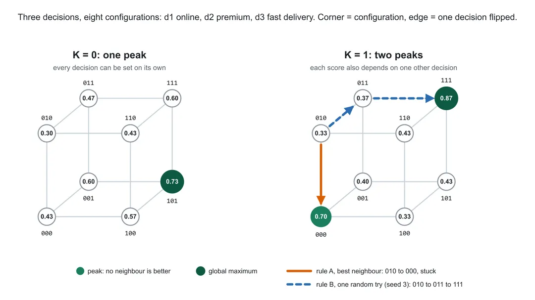
A peak, or local optimum, is a corner where every connected corner is lower. With K = 0 there is one, 101. With K = 1 there are two: 000 at 0.70 and 111 at 0.87.
Why the firm gets stuck
Suppose the firm is the local shop, 000, and tries only going online, which gives 100:
| at 000 | at 100 | what happened | |
|---|---|---|---|
| score of online | 0.8 | 0.2 | online without premium is a price war |
| score of premium | 0.7 | 0.7 | unchanged, it does not look at online |
| score of delivery | 0.6 | 0.1 | slow delivery is a problem now that the firm is online |
| fitness | 0.70 | 0.33 |
One decision changed and two scores moved, because delivery's score looks at online. In case 1 a flip could only change its own score. The move looks like a mistake, so the firm reverses it. Trying only premium or only fast delivery goes the same way. The firm concludes it is already at its best and stays at 0.70. The 0.87 exists, but it is only reachable by changing everything at once.
That is a rugged landscape with a local optimum, and it is the core phenomenon that Levinthal, Rivkin and Siggelkow and Wall study: interdependent decisions make step-by-step improvement get trapped on a mediocre peak.
How many numbers a landscape needs
A landscape is nothing more than its random payoff numbers; the fitness values, the peaks and the getting stuck are all computed from them by lookup and averaging. Each decision's table needs one number for every combination of the decisions it looks at: itself plus K others, so 2^(K+1) rows.
| K | a score looks at | rows per table |
|---|---|---|
| 0 | itself | 2 |
| 1 | itself and 1 other | 4 |
| 2 | itself and 2 others | 8 |
| 3 | itself and 3 others | 16 |
In total N × 2^(K+1) numbers:
| numbers to draw | |
|---|---|
| our firm, N = 3, K = 1 | 3 × 4 = 12 |
| Levinthal (1997), N = 10, K = 0 | 10 × 2 = 20 |
| N = 10, K = 5 | 10 × 64 = 640 |
| Rivkin and Siggelkow, N = 12, K = 11 | 12 × 4,096 = 49,152 |
At K = N - 1 every score looks at every decision; flipping any one decision changes every score and the landscape is as rugged as it can be. At K = 0 there is one smooth hill. K is the dial between the two.
Who looks at whom: the interaction matrix
In words, online looks at premium, premium at delivery and delivery at online. The papers write the same information as a grid. A row says what a score depends on, a column says which scores change when that decision flips:
           d1 d2 d3
  score 1   X  X  .
  score 2   .  X  X
  score 3   X  .  X
Every row has an X on the diagonal, because a score always looks at its own decision, and K is the number of X's in a row minus that one. Column d1 has X's in rows 1 and 3, which is exactly why flipping "online" moved the online score and the delivery score in the table above.
The grid matters beyond K. Here are two ways to fill a 6 × 6 grid with K = 2, so every row has three X's:
next-K                              random-K (Kauffman's original)
           d1 d2 d3 d4 d5 d6                   d1 d2 d3 d4 d5 d6
  score 1   X  X  X  .  .  .          score 1   X  X  .  .  X  .
  score 2   .  X  X  X  .  .          score 2   .  X  X  X  .  .
  score 3   .  .  X  X  X  .          score 3   X  .  X  .  X  .
  score 4   .  .  .  X  X  X          score 4   X  .  X  X  .  .
  score 5   X  .  .  .  X  X          score 5   .  .  X  X  X  .
  score 6   X  X  .  .  .  X          score 6   .  .  X  X  .  X
The rows are equally full, the columns are not. In the next-K grid every decision affects exactly three scores. In the random grid, d3 affects five scores and d6 only its own: flipping d3 shakes almost the whole firm, flipping d6 disturbs nothing else. The organization papers go further and give departments their own blocks of the grid, which is where decomposability, coordination and incentives come in. That is why nkscape stores the matrix as a real object and builds every landscape from one.
One seed, several random ingredients
A random number generator is a long list of numbers that is already fixed, with a bookmark in it. Every draw reads from the bookmark and moves it forward. The trap is one shared generator for everything. Build three landscapes and run a search on each, all drawing from one generator, and then change how many numbers the search uses:
search uses 2 random numbers per run:        search uses 5 random numbers per run:
  landscape 0: [0.77 0.44 0.86]                landscape 0: [0.77 0.44 0.86]
  landscape 1: [0.98 0.76 0.79]                landscape 1: [0.13 0.45 0.37]
  landscape 2: [0.37 0.93 0.64]                landscape 2: [0.55 0.06 0.83]
Landscapes 1 and 2 are different, although the seed and the landscape code did not change. The search moved the bookmark, so the next landscape started reading somewhere else. Compare two search strategies over a thousand landscapes this way and part of the difference you measure is one strategy getting easier landscapes.
The fix is separate streams. parent.spawn(2) gives two children that are statistically independent, and the same seed always gives the same children. In nkscape every random ingredient gets its own stream: the matrix, the tables, every agent, every rule. That is why an agent walks the same way alone as in a crowd.
How rugged: the number of peaks
For a small landscape the library can hold the fitness of every configuration at once, as an array with one axis of length 2 per decision, built by broadcasting the payoff tables. For the firm:
fitness cube (position = configuration):
[[[0.7  0.4 ]
  [0.33 0.37]]

 [[0.33 0.43]
  [0.43 0.87]]]
peaks: [[0, 0, 0], [1, 1, 1]] | count: 2
global maximum: 0.87
With that, counting peaks is cheap, and the first thing to look at is how the count grows with K. Here are 200 random landscapes per K with N = 10:
| K | peaks, mean | fewest | most |
|---|---|---|---|
| 0 | 1.0 | 1 | 1 |
| 1 | 3.4 | 1 | 15 |
| 2 | 7.7 | 1 | 25 |
| 3 | 13.8 | 4 | 25 |
| 4 | 21.8 | 10 | 34 |
| 5 | 32.6 | 23 | 45 |
| 6 | 44.0 | 32 | 58 |
| 7 | 58.3 | 45 | 72 |
| 8 | 74.3 | 59 | 88 |
| 9 | 92.7 | 74 | 110 |
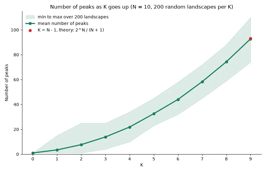
At K = N - 1 theory says 2^N / (N + 1) peaks on average, 93.1 for N = 10, and the measured 92.7 sits right there. The 2,000 landscapes took 0.6 seconds. The cube costs 8 bytes per configuration, so memory is what limits it: N = 24 needs 0.13 GB, N = 30 needs 8.6 GB, which is why the library refuses above 24 unless you raise the limit.
Walking the landscape
A period is one tick of the clock. In each period an agent looks around, decides, and moves or stays. Here are two hand-written rules, both starting at 010 on the firm's landscape, whose peaks are 000 at 0.70 and 111 at 0.87.
Rule A, best neighbour: each period, look at all three neighbours and move to the best one if it beats staying.
at 010 (0.33)  sees 110=0.43, 000=0.70, 011=0.37  ->  move to 000
at 000 (0.70)  sees 100=0.33, 010=0.33, 001=0.40  ->  nothing better -> stay
at 000 (0.70)  sees 100=0.33, 010=0.33, 001=0.40  ->  nothing better -> stay
After one move the agent stays at 000 forever. It took the largest immediate gain and that put it on the lower peak.
Rule B, one random try: each period, pick one decision at random and flip it if the result is better.
seed 1                                        seed 3
at 010 (0.33) tries d1: 000=0.70 -> move      at 010 (0.33) tries d2: 011=0.37 -> move
at 000 (0.70) tries d1: 010=0.33 -> stay      at 011 (0.37) tries d0: 111=0.87 -> move
at 000 (0.70) tries d2: 001=0.40 -> stay      at 111 (0.87) tries d0: 011=0.37 -> stay
Both runs start at the same place with the same rule and end on different peaks. With seed 1 the agent happened to try d1 first and landed on the lower peak. With seed 3 it tried d2 first, took a small gain from 0.33 to 0.37, and from there the path to the global peak was open. Two things follow: agents need randomness, and it has to be seeded, because the seed decides which peak the agent reaches. And greedy is not always better; rule A's bigger first step led to the worse peak.
One hand-made landscape proves little, so here are both rules on 200 landscapes with N = 10 and K = 3, 50 random starts each, 10,000 walks per rule:
| Rule | final fitness / global max | reached the global max | periods until stuck |
|---|---|---|---|
| A, best neighbour | 0.935 | 23.7 % | 3.1 |
| B, one random try | 0.926 | 20.3 % | 21.5 |
Both rules get stuck below the top most of the time; only about one walk in five reaches the global maximum. That is the core finding of the rugged-landscape literature. Fitness is divided by the global maximum of each landscape, because raw fitness is not comparable across landscapes. And what an agent may do within one period, look at all neighbours or at one, is a modelling decision that every paper makes on its own, which is why in nkscape the agent defines its own period.
From the toy firm to Levinthal (1997)
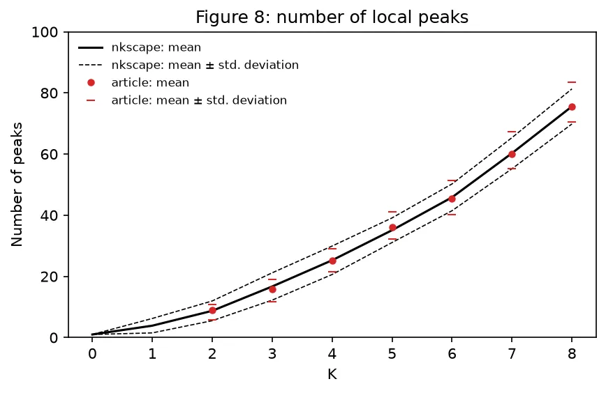
Levinthal's paper does exactly this with N = 10, a hundred organizations per landscape and a hundred landscapes, and adds long jumps, selection and a landscape that changes halfway. The notebook in the repository reproduces its Figures 1 to 9; the red dots are the values read off the figures in the article.
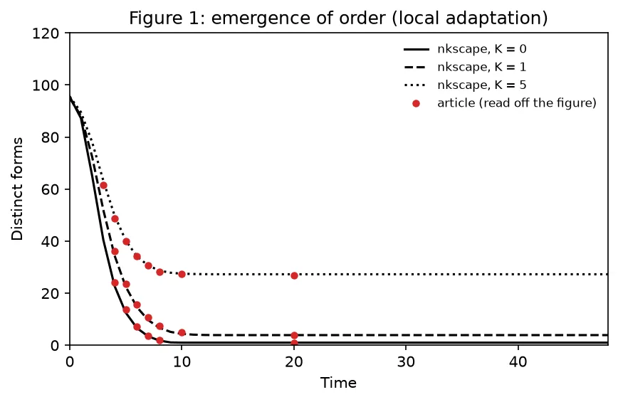
Some details are not in the article. The first version of my hill climber chose a better neighbour at random and was off by up to 19 forms in the early periods. Levinthal's original Turbo Pascal program is still online, and it settled it: neighbours are tried in a fixed order and the first better one is taken, which reproduces the figure. The program also answered how survival is decided, how newcomers are created and which noise formula Figure 9 needs.
What is in the library
Everything above: nk.Landscape holds the matrix and the tables, nk.Agent is a rule like A or B, nk.run runs the periods and nk.agents.HillClimber is the ready-made climber with Levinthal's long jumps. What is not in it yet, and what I want to add as time allows: departments that own subsets of the decisions, with the coordination modes and incentive schemes of Rivkin and Siggelkow (2003) and Wall (2016), satisficing agents, an experiment runner and plots.